Exploring the NOAA Storm Database focused on severe weather events
Lars Bartsch
04. März 2018
Synopsis
The U.S. National Oceanic and Atmospheric Administration’s (NOAA) storm database is a suitable source for exploring major weather effects in order to priorize the right cases and related countermeasures. Looking at the consequences of severe weather conditions, we focus on population health and economic issues that are sufficiently measurable. It can be narrowed down to two key questions to be answered:
1. Which types of weather events are most harmful with
respect to population health?
2. Which types of weather events have the greatest economic
consequences?
The database mentioned above consists of a time series starting in the year 1950 and ending in November 2011. It forms a broad basis for our following analysis. This is carries out with R in a reproducible way, which means that every step of the data retrieval, reshaping calculation and presenting is completely comprehensible.
Here we go..
Setup
knitr::opts_chunk$set(echo = TRUE, cache = TRUE, message = FALSE, warnings = FALSE)
options(scipen=999) # non-scientific number format
options(digits=2) # round to 2 decimal places
library(tidyverse) # includes ggplot2, tibble, tidyr, readr, purrr, dplyr
Data Processing
Raw Data Retrival
The data for this assignment come in the form of a
comma-separated-value file compressed via the bzip2 algorithm. At the
first step, we need to retrieve the raw data from the online source and
decompress it to a raw dataset called storm_raw. Due to the
size of the data, we use the more efficient method read_csv
from the tidyverse package to import the data as a tibble.
Moreover, we use cache = TRUE as standard chunk set.
Check Import
Secondly, we want to check the import.
## [1] "spec_tbl_df" "tbl_df" "tbl" "data.frame"## [1] "STATE__" "BGN_DATE" "BGN_TIME" "TIME_ZONE" "COUNTY" "COUNTYNAME" "STATE" "EVTYPE" "BGN_RANGE" "BGN_AZI" "BGN_LOCATI"
## [12] "END_DATE" "END_TIME" "COUNTY_END" "COUNTYENDN" "END_RANGE" "END_AZI" "END_LOCATI" "LENGTH" "WIDTH" "F" "MAG"
## [23] "FATALITIES" "INJURIES" "PROPDMG" "PROPDMGEXP" "CROPDMG" "CROPDMGEXP" "WFO" "STATEOFFIC" "ZONENAMES" "LATITUDE" "LONGITUDE"
## [34] "LATITUDE_E" "LONGITUDE_" "REMARKS" "REFNUM"## # A tibble: 3 × 37
## STATE__ BGN_DATE BGN_TIME TIME_ZONE COUNTY COUNTYNAME STATE EVTYPE BGN_RANGE BGN_AZI BGN_LOCATI END_DATE END_TIME COUNTY_END COUNTYENDN END_RANGE END_AZI
## <dbl> <chr> <chr> <chr> <dbl> <chr> <chr> <chr> <dbl> <chr> <chr> <chr> <chr> <dbl> <lgl> <dbl> <chr>
## 1 1 4/18/19… 0130 CST 97 MOBILE AL TORNA… 0 <NA> <NA> <NA> <NA> 0 NA 0 <NA>
## 2 1 4/18/19… 0145 CST 3 BALDWIN AL TORNA… 0 <NA> <NA> <NA> <NA> 0 NA 0 <NA>
## 3 1 2/20/19… 1600 CST 57 FAYETTE AL TORNA… 0 <NA> <NA> <NA> <NA> 0 NA 0 <NA>
## # ℹ 20 more variables: END_LOCATI <chr>, LENGTH <dbl>, WIDTH <dbl>, F <dbl>, MAG <dbl>, FATALITIES <dbl>, INJURIES <dbl>, PROPDMG <dbl>, PROPDMGEXP <chr>,
## # CROPDMG <dbl>, CROPDMGEXP <chr>, WFO <chr>, STATEOFFIC <chr>, ZONENAMES <chr>, LATITUDE <dbl>, LONGITUDE <dbl>, LATITUDE_E <dbl>, LONGITUDE_ <dbl>,
## # REMARKS <chr>, REFNUM <dbl>## spc_tbl_ [902,297 × 37] (S3: spec_tbl_df/tbl_df/tbl/data.frame)
## $ STATE__ : num [1:902297] 1 1 1 1 1 1 1 1 1 1 ...
## $ BGN_DATE : chr [1:902297] "4/18/1950 0:00:00" "4/18/1950 0:00:00" "2/20/1951 0:00:00" "6/8/1951 0:00:00" ...
## $ BGN_TIME : chr [1:902297] "0130" "0145" "1600" "0900" ...
## $ TIME_ZONE : chr [1:902297] "CST" "CST" "CST" "CST" ...
## $ COUNTY : num [1:902297] 97 3 57 89 43 77 9 123 125 57 ...
## $ COUNTYNAME: chr [1:902297] "MOBILE" "BALDWIN" "FAYETTE" "MADISON" ...
## $ STATE : chr [1:902297] "AL" "AL" "AL" "AL" ...
## $ EVTYPE : chr [1:902297] "TORNADO" "TORNADO" "TORNADO" "TORNADO" ...
## $ BGN_RANGE : num [1:902297] 0 0 0 0 0 0 0 0 0 0 ...
## $ BGN_AZI : chr [1:902297] NA NA NA NA ...
## $ BGN_LOCATI: chr [1:902297] NA NA NA NA ...
## $ END_DATE : chr [1:902297] NA NA NA NA ...
## $ END_TIME : chr [1:902297] NA NA NA NA ...
## $ COUNTY_END: num [1:902297] 0 0 0 0 0 0 0 0 0 0 ...
## $ COUNTYENDN: logi [1:902297] NA NA NA NA NA NA ...
## $ END_RANGE : num [1:902297] 0 0 0 0 0 0 0 0 0 0 ...
## $ END_AZI : chr [1:902297] NA NA NA NA ...
## $ END_LOCATI: chr [1:902297] NA NA NA NA ...
## $ LENGTH : num [1:902297] 14 2 0.1 0 0 1.5 1.5 0 3.3 2.3 ...
## $ WIDTH : num [1:902297] 100 150 123 100 150 177 33 33 100 100 ...
## $ F : num [1:902297] 3 2 2 2 2 2 2 1 3 3 ...
## $ MAG : num [1:902297] 0 0 0 0 0 0 0 0 0 0 ...
## $ FATALITIES: num [1:902297] 0 0 0 0 0 0 0 0 1 0 ...
## $ INJURIES : num [1:902297] 15 0 2 2 2 6 1 0 14 0 ...
## $ PROPDMG : num [1:902297] 25 2.5 25 2.5 2.5 2.5 2.5 2.5 25 25 ...
## $ PROPDMGEXP: chr [1:902297] "K" "K" "K" "K" ...
## $ CROPDMG : num [1:902297] 0 0 0 0 0 0 0 0 0 0 ...
## $ CROPDMGEXP: chr [1:902297] NA NA NA NA ...
## $ WFO : chr [1:902297] NA NA NA NA ...
## $ STATEOFFIC: chr [1:902297] NA NA NA NA ...
## $ ZONENAMES : chr [1:902297] NA NA NA NA ...
## $ LATITUDE : num [1:902297] 3040 3042 3340 3458 3412 ...
## $ LONGITUDE : num [1:902297] 8812 8755 8742 8626 8642 ...
## $ LATITUDE_E: num [1:902297] 3051 0 0 0 0 ...
## $ LONGITUDE_: num [1:902297] 8806 0 0 0 0 ...
## $ REMARKS : chr [1:902297] NA NA NA NA ...
## $ REFNUM : num [1:902297] 1 2 3 4 5 6 7 8 9 10 ...
## - attr(*, "spec")=
## .. cols(
## .. STATE__ = col_double(),
## .. BGN_DATE = col_character(),
## .. BGN_TIME = col_character(),
## .. TIME_ZONE = col_character(),
## .. COUNTY = col_double(),
## .. COUNTYNAME = col_character(),
## .. STATE = col_character(),
## .. EVTYPE = col_character(),
## .. BGN_RANGE = col_double(),
## .. BGN_AZI = col_character(),
## .. BGN_LOCATI = col_character(),
## .. END_DATE = col_character(),
## .. END_TIME = col_character(),
## .. COUNTY_END = col_double(),
## .. COUNTYENDN = col_logical(),
## .. END_RANGE = col_double(),
## .. END_AZI = col_character(),
## .. END_LOCATI = col_character(),
## .. LENGTH = col_double(),
## .. WIDTH = col_double(),
## .. F = col_double(),
## .. MAG = col_double(),
## .. FATALITIES = col_double(),
## .. INJURIES = col_double(),
## .. PROPDMG = col_double(),
## .. PROPDMGEXP = col_character(),
## .. CROPDMG = col_double(),
## .. CROPDMGEXP = col_character(),
## .. WFO = col_character(),
## .. STATEOFFIC = col_character(),
## .. ZONENAMES = col_character(),
## .. LATITUDE = col_double(),
## .. LONGITUDE = col_double(),
## .. LATITUDE_E = col_double(),
## .. LONGITUDE_ = col_double(),
## .. REMARKS = col_character(),
## .. REFNUM = col_double()
## .. )
## - attr(*, "problems")=<externalptr>At a first glance, everything looks properly imported. We’ve got a tibble with 902297 observations of 37 variables. Every variable seems to be labeled.
Select relevant variables
Refering to our research questions, we identify all relevant vaiables
derived from names() and the online documentation provided
above. We cut them into the dataset storm_select via
select using a single pipe.
storm_select <- storm_raw %>% select("EVTYPE", "FATALITIES", "INJURIES", "PROPDMG", "PROPDMGEXP", "CROPDMG", "CROPDMGEXP")The new dataset consists of only 7 variables, i. e.:
- event type,
- fatalities,
- injuries,
- property damage,
- property damage exponent,
- crop damage and
- crop damage exponent.
Convert damage codes into real expenses
To do so, we initiate a loop — one for property and one for crop —
and input the code-value pairs (from variable PROPDMGEXP
and CROPDMGEXP, resp.), e. g. H100 means code
“H” that stands for “factor hundred”. By this, we are able to calculate
the resulting variable “PROPDMGREAL” with only one loop using the method
substr. The calculation is a simple multiplication with the
variables PROPDMG and CROPDMG, resp. Inside
the loop, the parts are binded into a new dataset
storm_convert that is initiated in advance. Last but not
least, we tidy up some patterns in variable EVTYPE.
storm_convert = NULL

for(n in c("H100", "K1000", "M1000000", "B1000000000")) {
  part <- storm_select %>%
          filter(PROPDMGEXP == substr(n, 1, 1) | CROPDMGEXP == substr(n, 1, 1)) %>%
          mutate(PROPDMGREAL = PROPDMG * as.numeric(substr(n, 2, nchar(n)))) %>%
          mutate(CROPDMGREAL = CROPDMG * as.numeric(substr(n, 2, nchar(n))))

  storm_convert <- rbind(storm_convert, part)
}

ev_types <- tolower(storm_convert$EVTYPE)
ev_types <- gsub("[[:blank:][:punct:]+]", " ", ev_types)
storm_convert$EVTYPE <- ev_types
In result, we’ve got got a tibble storm_convert with
444510 observations of 9 variables. In the last data processing step, we
remove the dataset that are not needed any more, and have a look at our
neat processed tibble to go further.
## [1] "tbl_df" "tbl" "data.frame"## [1] "EVTYPE" "FATALITIES" "INJURIES" "PROPDMG" "PROPDMGEXP" "CROPDMG" "CROPDMGEXP" "PROPDMGREAL" "CROPDMGREAL"## # A tibble: 3 × 9
## EVTYPE FATALITIES INJURIES PROPDMG PROPDMGEXP CROPDMG CROPDMGEXP PROPDMGREAL CROPDMGREAL
## <chr> <dbl> <dbl> <dbl> <chr> <dbl> <chr> <dbl> <dbl>
## 1 thunderstorm winds 0 0 5 H 0 <NA> 500 0
## 2 thunderstorm winds 0 0 5 H 0 <NA> 500 0
## 3 thunderstorm winds 0 0 2 H 0 <NA> 200 0## tibble [444,510 × 9] (S3: tbl_df/tbl/data.frame)
## $ EVTYPE : chr [1:444510] "thunderstorm winds" "thunderstorm winds" "thunderstorm winds" "thunderstorm winds" ...
## $ FATALITIES : num [1:444510] 0 0 0 0 0 0 0 0 0 0 ...
## $ INJURIES : num [1:444510] 0 0 0 0 0 2 15 0 2 2 ...
## $ PROPDMG : num [1:444510] 5 5 2 3 5 5 25 2.5 25 2.5 ...
## $ PROPDMGEXP : chr [1:444510] "H" "H" "H" "H" ...
## $ CROPDMG : num [1:444510] 0 0 0 0 0 0 0 0 0 0 ...
## $ CROPDMGEXP : chr [1:444510] NA NA NA NA ...
## $ PROPDMGREAL: num [1:444510] 500 500 200 300 500 500 25000 2500 25000 2500 ...
## $ CROPDMGREAL: num [1:444510] 0 0 0 0 0 0 0 0 0 0 ...Results
Here we are going to present the results by following two major questions:
1. Across the United States, which types of events (as indicated in the EVTYPE variable) are most harmful with respect to population health?
2. Across the United States, which types of events have the greatest economic consequences?
First of it, we summarise the processed data types using
summarise:
storm_convert %>% summarise(sum(FATALITIES))
storm_convert %>% summarise(sum(INJURIES))

storm_convert %>% summarise(sum(PROPDMGREAL))
storm_convert %>% summarise(sum(CROPDMGREAL))
In summary we find a total of 10791 fatalities and 136381 injuries. Furthermore, we find a total of 1057927616250 Dollars in property damage and a total of 1807269231390 Dollars in crop damage.
Regarding the most harmful events to population health, we can show a
barplot next. Threrefore, we get plot datasets storm_sum
for fatalities and injuries grouped by event type. After ordering we use
ggplot to construct the plots of the TOP 6.
storm_sum <- storm_convert %>%
              group_by(EVTYPE) %>%
              summarise(FATALITIES = sum(FATALITIES)) %>%
              arrange(desc(FATALITIES))

storm_sum$EVTYPE <- factor(storm_sum$EVTYPE, levels = storm_sum$EVTYPE[order(storm_sum$FATALITIES, decreasing = TRUE)])
ggplot(data = head(storm_sum, n = 6), aes(x = EVTYPE, y = FATALITIES)) + geom_bar(stat = "identity") + xlab("Events") + ylab("Fatality Count")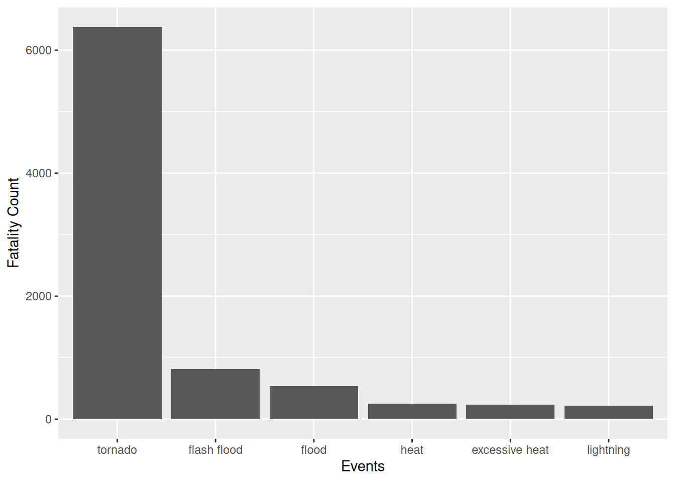
storm_sum <- storm_convert %>%
              group_by(EVTYPE) %>%
              summarise(INJURIES = sum(INJURIES)) %>%
              arrange(desc(INJURIES))

storm_sum$EVTYPE <- factor(storm_sum$EVTYPE, levels = storm_sum$EVTYPE[order(storm_sum$INJURIES, decreasing = TRUE)])
ggplot(data = head(storm_sum, n = 6), aes(x = EVTYPE, y = INJURIES)) + geom_bar(stat = "identity") + xlab("Events") + ylab("Injury Count")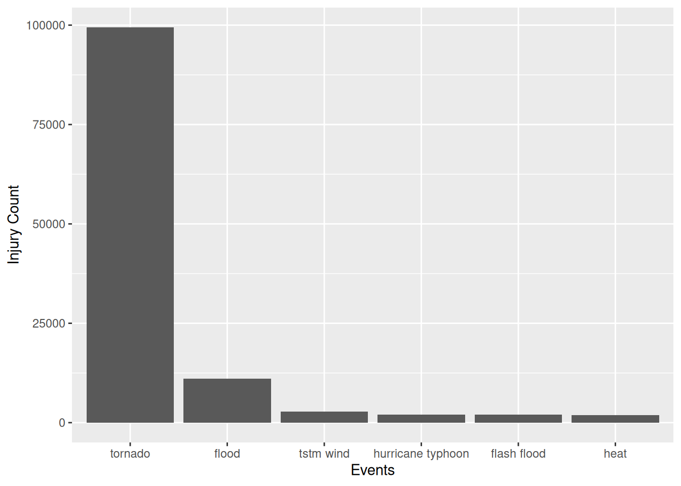
Now we finish our results by showing the types of events that have
the greatest economic consequences. For doing this, we sum up the damage
values of property and crop with mutate.
storm_sum <- storm_convert %>%
              mutate(TOTALREAL = PROPDMGREAL + CROPDMGREAL) %>%
              group_by(EVTYPE) %>%
              summarise(TOTALREAL = sum(TOTALREAL)) %>%
              arrange(desc(TOTALREAL))

storm_sum$EVTYPE <- factor(storm_sum$EVTYPE, levels = storm_sum$EVTYPE[order(storm_sum$TOTALREAL, decreasing = TRUE)])
ggplot(data = head(storm_sum, n = 6), aes(x = EVTYPE, y = TOTALREAL)) + geom_bar(stat = "identity") + xlab("Events") + ylab("Total Damage in Dollars")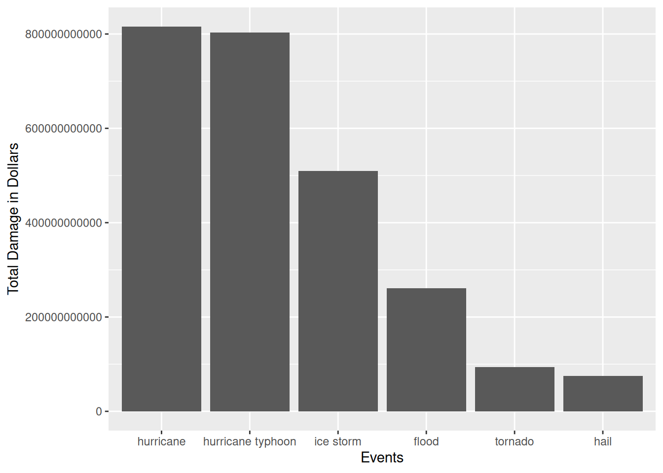
Conclusion:
As the results show at first, tornados, flash floods, floods, heat,
excessive heat and lightning are the most deadly weather events in
decreasing order. That is the most severe factor regarding public
health. Secondly, tornados, floods, heavy winds, hurricane typhoons,
flash floods and heat are the main causes of weather-related injuries in
decreasing order.
When it comes to economic consequences, the picture slightly differs. Here the most severe weather events are hurricanes, hurricane typhoons, ice storms, floods, tornados and hails in decreasing order.
Appendix
Review criteria
- Has either a (1) valid RPubs URL pointing to a data analysis document for this assignment been submitted; or (2) a complete PDF file presenting the data analysis been uploaded?
- Is the document written in English?
- Does the analysis include description and justification for any data transformations?
- Does the document have a title that briefly summarizes the data analysis?
- Does the document have a synopsis that describes and summarizes the data analysis in less than 10 sentences?
- Is there a section titled “Data Processing” that describes how the data were loaded into R and processed for analysis?
- Is there a section titled “Results” where the main results are presented?
- Is there at least one figure in the document that contains a plot?
- Are there at most 3 figures in this document?
- Does the analysis start from the raw data file (i.e. the original .csv.bz2 file)?
- Does the analysis address the question of which types of events are most harmful to population health?
- Does the analysis address the question of which types of events have the greatest economic consequences?
- Do all the results of the analysis (i.e. figures, tables, numerical summaries) appear to be reproducible?
- Do the figure(s) have descriptive captions (i.e. there is a description near the figure of what is happening in the figure)?
- As far as you can determine, does it appear that the work submitted for this project is the work of the student who submitted it?
Build with
## R version 4.3.3 (2024-02-29)
## Platform: x86_64-pc-linux-gnu (64-bit)
## Running under: Manjaro Linux
##
## Matrix products: default
## BLAS:   /usr/lib/libblas.so.3.12.0
## LAPACK: /usr/lib/liblapack.so.3.12.0
##
## locale:
##  [1] LC_CTYPE=de_DE.UTF-8       LC_NUMERIC=C               LC_TIME=de_DE.UTF-8        LC_COLLATE=de_DE.UTF-8     LC_MONETARY=de_DE.UTF-8
##  [6] LC_MESSAGES=de_DE.UTF-8    LC_PAPER=de_DE.UTF-8       LC_NAME=C                  LC_ADDRESS=C               LC_TELEPHONE=C
## [11] LC_MEASUREMENT=de_DE.UTF-8 LC_IDENTIFICATION=C
##
## time zone: Europe/Berlin
## tzcode source: system (glibc)
##
## attached base packages:
## [1] stats     graphics  grDevices utils     datasets  methods   base
##
## other attached packages:
##  [1] highcharter_0.9.4  kableExtra_1.4.0   DT_0.32            stopwords_2.3      tidytext_0.4.1     RColorBrewer_1.1-3 ggthemes_5.1.0
##  [8] lubridate_1.9.3    forcats_1.0.0      stringr_1.5.1      dplyr_1.1.4        purrr_1.0.2        readr_2.1.5        tidyr_1.3.1
## [15] tibble_3.2.1       ggplot2_3.5.0      tidyverse_2.0.0
##
## loaded via a namespace (and not attached):
##  [1] tidyselect_1.2.1  viridisLite_0.4.2 farver_2.1.1      fastmap_1.1.1     janeaustenr_1.0.0 digest_0.6.35     timechange_0.3.0  lifecycle_1.0.4
##  [9] tokenizers_0.3.0  magrittr_2.0.3    compiler_4.3.3    rlang_1.1.3       sass_0.4.9        tools_4.3.3       igraph_2.0.3      utf8_1.2.4
## [17] yaml_2.3.8        data.table_1.15.4 knitr_1.45        labeling_0.4.3    htmlwidgets_1.6.4 bit_4.0.5         curl_5.2.1        xml2_1.3.6
## [25] TTR_0.24.4        withr_3.0.0       grid_4.3.3        fansi_1.0.6       xts_0.13.2        colorspace_2.1-0  scales_1.3.0      cli_3.6.2
## [33] rmarkdown_2.26    crayon_1.5.2      generics_0.1.3    rlist_0.4.6.2     rstudioapi_0.16.0 tzdb_0.4.0        cachem_1.0.8      assertthat_0.2.1
## [41] parallel_4.3.3    vctrs_0.6.5       Matrix_1.6-5      jsonlite_1.8.8    hms_1.1.3         bit64_4.0.5       crosstalk_1.2.1   systemfonts_1.0.6
## [49] fontawesome_0.5.2 jquerylib_0.1.4   quantmod_0.4.26   glue_1.7.0        stringi_1.8.3     gtable_0.3.4      munsell_0.5.0     pillar_1.9.0
## [57] htmltools_0.5.8   R6_2.5.1          vroom_1.6.5       evaluate_0.23     lattice_0.22-5    highr_0.10        backports_1.4.1   SnowballC_0.7.1
## [65] broom_1.0.5       bslib_0.7.0       Rcpp_1.0.12       svglite_2.1.3     xfun_0.43         zoo_1.8-12        pkgconfig_2.0.3
Dieses Werk ist lizenziert unter einer Creative Commons Attribution-ShareAlike 4.0 International License.